Lewis Reeves
ELEC 2120 Signals & Systems
11/6/2024
Lab 9: Convolution TIMS Week 2
Introduction:
This lab continues on the previous week’s understanding of convolution to further students’ understanding. The lab expands on the concept of superposition to demonstrate the convolution of signals.
Procedure:
1. Unit Pulse Response
First, the circuit from the previous week shown in Figure 1 is constructed on the TIMS. Both clocks are connected to 1kHz. The SFP gain is set to b0 = 0.3, b1 = 0.5, and b2 = -0.2. The input pulses once which causes the output to pulse three separate times scaled according to the SFP gains in order. An electrical component that is responsible for the presence of delayed energy could be a flip flop.
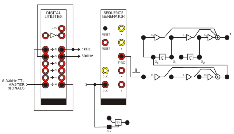
Figure 1 – Convolution Wiring Diagram
2. The Superposition Sum
The equation of discrete convolution is displayed as Equation 1. The superposition sum is the sum of each signal delayed and scaled in order of their delay. Next, the SEQUENCE GENERATOR clock rate is switched to the 500Hz input. The input and output are examined to see that they match the input and output of the previous week. Based on the results, the expected result of having four back-to-back clock pulses would be an output of four input signals delayed by one, two, three, and four all added together. This could be simulated by changing the clock to 250Hz for the SEQUENCE GENERATOR.
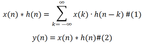
Equation 1 – Discrete Convolution
3. Rectified Sinewave at Input
The system is then configured according to Figure 2. This rectified output will be the input of our signal. Each output (b0-b2) is individually recorded along with the final output. The handout with the resulting signals is displayed in Figure 3. The error in y[0] was 0.1 – (0.15 + 0.05) = -0.1V. The error for y[1] was 1.00 – (0.83 + 0.2 + 0.05) = -0.08V. The error for y[2] was 2.3 – (1.1 + 1.3 – 0.1) = 0.00V. The equation for y[1] = 0.3 x x[1] + 0.5 x x[0] + -0.2 x x[-1]. The equation for y[2] = 0.3 x x[2] + 0.5 x x[1] + -0.2 x x[0]. Th equation for y[6] = 0.3 x x[6] + 0.5 x x[5] + -0.2 x x[4]
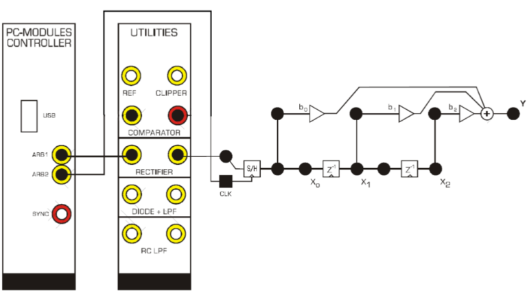
Figure 2 – Rectified Sinewave

Figure 3 – Convolution Handout
Conclusions:
This lab further expanded on the understanding of superposition and convolution from the previous week. The individual components of the superposition signal are measured, and their sums are close to the superimposed output signal. Some error is involved since the signals pass through a system, but the results are close enough. I enjoyed seeing how adding the individual signals together gives you the convoluted resulting output. This lab went well for most of it, but remembering to switch clocks from step to step caused some problems which had to take up time diagnosing. I would improve this lab by adding a sample of the convolution handout but with a different signal.