Lewis Reeves
ELEC 2120 Signals & Systems
10/1/2024
Lab 6: System Linearity TIMS
Introduction:
This lab demonstrates examples of signals with linearity and time-invariance. Throughout the lab, each signal will be analyzed and determined to be linear or time-invariant. This experiment introduces the VCO, Multiplier, Variable DC, and Laplace V2 modules to created the systems. A system is found to be linear if it follows both the scaling and the additive criteria.
Procedure:
A.1 Comparator
First, the VCO and Utilities modules are inserted into the TIMS. The VCO sin(t) output is connected to the Buffer Amplifier input A and to the input of Frequency Counter. The Buffer Amplifier output (k1A) to the Utilities module Comparator input and to scope ChA. The Utilities Clipper output is connected to scope ChB.
In the PicoScope software, Channel B is turned on to auto. Channel B and Channel A are turned to DC coupling. The time base is set to 500us/div, and the trigger is set to auto. The VCO f knob is adjusted to 1000 Hz. The Channel A signal is observed while the Buffer Amplifier gain k1 is adjusted to 1Vpp for Chael A. Next, the Buffer Amplifier gain k1 is adjusted and the peak to peak output voltages are recorded in the chart in Figure 1.
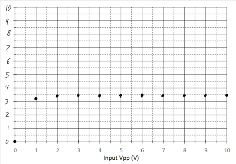
Figure 1 – Comparator Vpp Output vs. Input
This system is not linear because it does not follow the scaling property.
2. Recifier
For the rectifier, the Buffer Amplifier output k1A is connected to the Utilities module rectifier input and to scope ChA. Then scope ChB is connected to the Utilities module rectifier output. The VCO f knob is adjusted to 1000 Hz. The ChA signal is observed while the Buffer Amplifier gain k1 is adjusted to 1Vpp for ChA. The input signal amplitude is sdjusted 1Vpp at a time, and the resulting output is recorded on the graph in Figure 2.
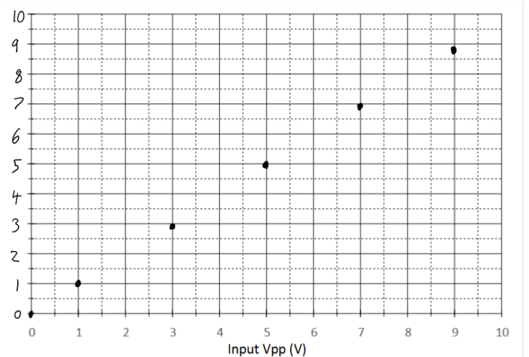
Figure 2 – Rectifier Vpp Output vs. Input
This system is linear because it does follow the scaling property.
3. Multiplier
Next, the VCO output is connected to the Buffer Amplifier input and the Frequency Counter with the VCO knob set to 1 kHz. The Bugger Amplifier input is connected to both the inputs of Multiplier and ChA. The Multiplier output is connected to scope ChB.
In the PicoScope software, Channel B is turned on to Auto. The trigger is set to auto and the time base is set to 500us/div. The Buffer Amplifier k1 knob is adjusted to reach 1Vpp input. The results are recorded in Table 1 and graphed in Figure 3.
|
Input Amplitude |
Output Amplitude |
|
0.5 |
0.11V |
|
1.0 |
0.54V |
|
1.5 |
1.20V |
|
2.0 |
2.09V |
|
3.0 |
4.57V |
|
4.0 |
8.15V |
Table 1 – Multiplier Amplitude Output vs. Input
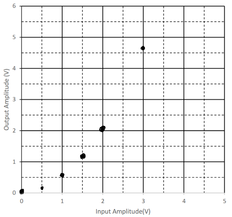
Figure 3 – Multiplier Amplitude Output vs. Input Graph
This system is not linear. The results do demonstrate the half angle formula (A^2)sin^2(t) = 1/2(A^2)(1-cos(2t)).
B.1 DC Control
Now, the VCO gain and f knobs are turned to about the center. The Variable DC output is connected to the input of VCO and scope ChB. The VCO output is connected to the Frequency Counter and scope ChA.
In the PicoScope software, Channel B is turned on and both channels are set to DC coupling. The trigger is set to auto and the time base is changed to 500us/div. The DC knob is changed from -2V to 2V and each 1V increment is recorded in Table 2 and graphed in Figure 4.
|
DC value (V) |
Signal frequency (Hz) |
|
-2 |
1k |
|
-1 |
1k |
|
0 |
1k |
|
1 |
1k |
|
2 |
1k |
Table 2 – DC Control value and Signal Frequency
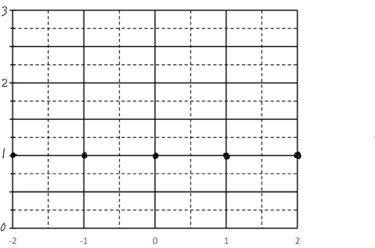
Figure 4 – DC Control Value vs. Signal Frequency
The system is linear.
2. Frequency Counter
Next, the Audio Oscillator sin(t) output is connected to input A of the Buffer Amplifier and the Frequency Counter Analog input. The Audio Oscillator sin(t) output is adjusted to 300 Hz on the Frequency Counter. The Buffer Amplifier k1A output is connected to the VCO Vin input and scope ChB. The VCO sin(t) output is connected to scope ChA.
Channel B is connected turned on to auto. Both channels are set to DC coupling and the time base is set to 500us/div. The triggering is set to single.
An application of this system could be a radio system.
C.1 The Integrator
For this section, the Audio Oscillator sin(t) output is connected to the Utilities Comparator input and the Frequency Counter Analog input. The Audio Oscillator f knob is set to 1 kHz. The Utilities output is connected to the Laplace V2 S1in and scope ChB. The Laplace V2 S1out is connected to scope ChA.
In the PicoScope software, Channel B is turned on to +/-5V, and both channels are connected to DC coupling. The time base is decreased to 500us/div and the triggering is set to auto. The result shows the integral value of the input signal.
2. Feedback System
The ARB2 output is connected to the scope ChA. The PicoScope software is adjusted to show the ARB2 signal. Then the S&S V2 SFP application is opened, and the tab labeled “Lab 3” is selected and loaded. The gain b1 is set to 1 and b2 is set to -1. The ARB2 output is now also connected to the b1 input of the Triple Adder. The ouput B of the Triple Adder V2 is connected to the S1in of Laplace V2. The S1out of Laplace V2 is connected to the b2 input of Triple Adder V2. The Triple Adder output B is connected to scope ChB.
In the PicoScope software, channel B is turned to auto, and the time scale is set to 200us/div. The triggering is set to single. The time constant is measured and found to be ~68.4us.
Conclusions:
This experiment was enjoyable because it showed how linear systems work vs non-linear. The experiment showed how an integrating system and Laplace system works which was interesting. This lab went well overall, but the DC control section was slightly confusing. This experiment could be improved by adding one or two figures of how to find the time constant in the last section.