Procedure:
1. For the differential equation:![]()
a. The corresponding transfer function is ![]()
b. The poles and zeros of this equation are p = -1, -3 and z = -3
c. The poles and zeros map is displayed in Figure 1
d. The system is asymptotically stable because it decays to zero as time continues. The system is stable because the poles are all less than zero, and the system is asymptotically stable because the poles are less than zero. The impulse response can be seen decaying to zero as time continues in Figure 2.


2. For the differential equation: ![]()
a. The corresponding transfer function is ![]()
b. The poles and zeros of this equation are p = -2 + j, -2 – j, 1 + j0 and z = 3, 4
c. The poles and zeros plot is displayed in Figure 3
d. The system is unstable because it grows unboundedly. The system is unstable because at least one pole is greater than zero. The impulse response is seen in Figure 4 to increase unboundedly.


3. For the differential equation: ![]()
a. The corresponding transfer function is ![]()
b. The poles and zeros of this equation are p = 0, -1, -2 + j, -2 – j1 and z = 7, 3
c. The poles and zeros plot is displayed in Figure 5
d. The system is stable because it is bounded by a constant. The system is not asymptotically stable because there is a pole that is equal to zero. The impulse response is seen in Figure 6 to be bound by a constant.


4. Design a third order transfer function that produces a stable impulse response. The function should have two zeros.
a. The function is defined as ![]()
b. The impulse response is displayed in Figure 7
c. The poles and zeros plot is displayed in Figure 8
d. The system is stable because the poles are less than or equal to zero. It is not asymptotically stable because there is a pole equal to zero.


5. Design a third order transfer function that produces an asymptotically stable impulse response. The function should have two zeros.
a. The function is defined as ![]()
b. The impulse response is displayed in Figure 9
c. The poles and zeros plot is displayed in Figure 10
d. The system is asymptotically stable because all the poles are less than zero.


6. Design a third order transfer function that produces an unstable impulse response. The function should have two zeros.
a. The function is defined as ![]()
b. The impulse response is displayed in Figure 13
c. The poles and zeros plot is displayed in Figure 14
d. The system is not stable because at least one pole is greater than zero.


7. The transfer function is found below.

8. The impulse response is ![]() .
.
a. The impulse response is displayed in Figure 15
b. The step response is displayed in Figure 16


10. As the resistance increases, the amount of oscillations decreases. As the resistance increases, the pole magnitude also decreases.
11.
a. The function ![]() is unstable because the poles and zeros are p = 1, -1 + j, -1 – j and z = 3, 4. One pole is greater than zero, causing the function to be unstable.
is unstable because the poles and zeros are p = 1, -1 + j, -1 – j and z = 3, 4. One pole is greater than zero, causing the function to be unstable.
b. The impulse response shown in Figure 18 shows that the function is unstable because it grows unboundedly.

12. The equation from part 11 can also be displayed as 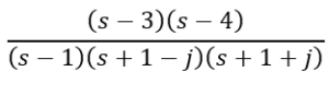
13.
a. The stable cancelled equation is now 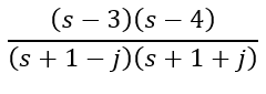
b. The multiplied out equation is 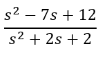
c. The impulse response of the system is displayed in Figure 19
d. The system is now asymptotically stable because all the real portions of the poles are less than zero. This is what was expected since the unstable pole was removed.
