Lab 11 – Lewis Portfolio

Lewis Reeves

ELEC 2120 Signals & Systems

11/19/2024

Lab 11: Complex Numbers TIMS

Introduction:

This experiment focuses on how imaginary numbers can be represented in a sinusoidal signal. The imaginary component will be graphed as the Y axis, and the real component is graphed on the X axis. Matlab will be used to solve for the phasor of rectangular coordinates and also solve for rectangular coordinates using the phasor.

Procedure:

A.1

First, the Triple Adder is inserted into the TIMS. The PC Modules Controller ARB1 output is connected to the Triple Adder f input and Scope CHA. The ARB2 output is connected to the g input of the adder ad Scope CHB.

In the PicoScope software CHB is turned on, and AC coupling is turned on for both channels. The time scale is set to 2ms/div, and the trigger is set to auto. In SFP, Lab 6 is selected, and the position of the Triple Adder is selected. The ARB1 is set to 1sin(t) shifted by 0, and the ARB2 is set to 1sin(t+90) which is shifted by 90. The sum of the ARB1 and ARB2 vectors is (1+0j) + (0 +1j) = (1+1j). This is the same as 2^(1/2)@45 degrees in polar form. The ARBs are loaded, and the signal is observed in the PicoScope.

The ARB2 phase is changed to -90 and loaded. The sum of the new ARB1 and ARB2 vectors is (1+0j) + (0 -1j) = (1-1j). This is the same as 2^(1/2)@-45 degrees in polar form.

Next, the PicoScope is set to display both the output signals and the XY view of the signals. Th XY plot displays a circle because the imaginary numbers are displayed on the Y axis and the real are displayed on the X axis. As the sinusoidal signal continues, the sum of the real and imaginary value moves in a circle as shown in Figure 1 because the signals are out of phase by 90 degrees. ARB 1 is disconnected from the Scope CHA, and the resulting XY graph displays a line from -1 to 1 on the Y axis. This is because the real component of the graph has been removed, and the output spans between -1j and 1j. ARB1 is reconnected, and ARB2 is disconnected from Scope CHB. The XY view displays a line from -1 to 1 on the X axis. This is because the imaginary component was removed, so the signal oscillates between -1 and 1 output.

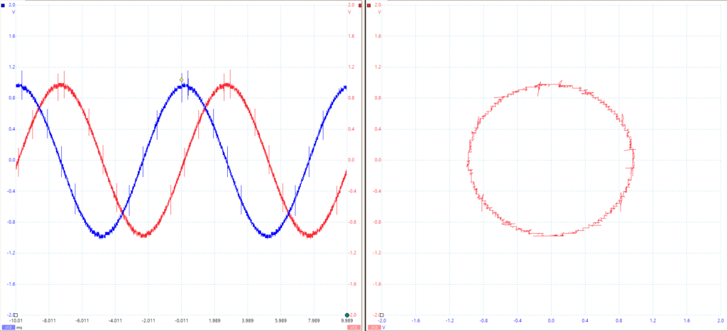
Figure 1 – XY and PicoScope Outputs

The ARB2 is reconnected to Scope CHB, and the SFP Triple Adder settings are adjusted so the Ref amplitude of ARB1 is 1 and the phase is -15 degrees. The Ref amplitude of ARB2 is set to 1.1 and the phase is set to -75 degrees. The ARB is then loaded. The graph is observed, and the resulting equation of each ARB is 1cos(t-15) for ARB1 and 1.2cos(t+75) for ARB2. The resulting signals and XY graph are displayed in Figure 2.

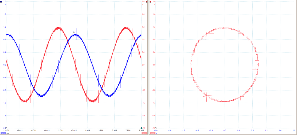
Figure 2 – XY and PicoScope Outputs of ARB1 = 1cos(t-15) and ARB2 = 1.2cos(t+75)

Now, Matlab will be used to convert polar coordinates into rectangular and also rectangular to polar. The functions [z] = pol2rec(x) and [x] = rec2pol(z) are used to call functions that will calculate this conversion for each. These Matlab functions are attached to the end of this lab report to be downloaded.

The ARB1 amplitude is reset to 1 and the phase to -15 degrees. The ARB 2 amplitude is set to 1.2 and the phase to 75 degrees. The CHB scope is connected to the f+g output, and the output is measured to be 1.501. The calculated result using the phasors was 1.562 amplitude at 35.2 degrees. The Ref amplitude of ARB1 is then set to 1 and the phase to 0 degrees. The Ref amplitude of ARB2 is set to 1.2 and the phase to 180 degrees. The ARB is then loaded. The output sum signal is 0.2@180 degrees. The phase of ARB2 is changed to -180 degrees, and the signal is observed again. The sum is still 0.2@180 degrees because 180 degrees is the same phase as -180 degrees. This is exactly what is expected mathematically.

The TIMS setup from the previous part is kept, and the ARB1 amplitude is set to 1, and the ARB 2 amplitude is set to 1 with phase 20 degrees. The Conjugate Phase mode is switched on. The ARB phasor is adjusted by steps of 30 degrees from 0 degrees all the way to 360 degrees, and the amplitude of each signal is measured and recorded in Table 1. The results are graphed in Matlab, and the result is shown in Figure 3.

Phase angle	Output amplitude
0	2.15
30	1.76
60	1.19
90	0.21
120	1.19
150	1.80
180	2.15
210	1.80
240	1.19
270	0.22
300	1.19
330	1.76
360	2.15

Table 1 – Conjugate Signal Amplitudes

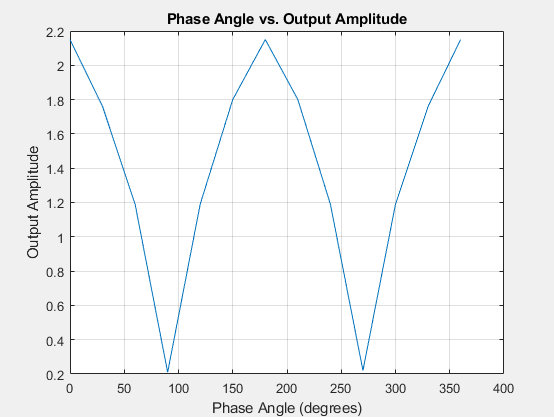
Figure 3 – Matlab Phase Angle vs. Output Amplitude Graph

Conclusions:

This lab successfully introduced how to work with imaginary numbers in signals. The signals were visualized as outputs using the imaginary values as the Y axis and the real values as the X axis. The calculation from polar to rectangular and from rectangular to polar coordinates was able to be done using Matlab. I enjoyed applying my Matlab understanding and TIMS understanding together to understand the imaginary components of signals more fully. I kept messing up my Matlab functions which took a few extra minutes to fix. I would improve this lab by having more Matlab examples to futher help students understand the signals.