Lewis Reeves
ELEC 2120 Signals & Systems
11/12/2024
Lab 10: Fourier Matlab
Introduction:
This lab covers how computers handle Fourier series as a function. Fourier series are infinite, so there has to be a way of calculating the Fourier series without it being infinite. The lab will demonstrate how to determine how accurate the series needs to be and find the right balance between loss of performance and a precise signal.
Procedure:
A.
1. What happens to the overall signal when harmonics are added?
– The signal becomes much more dense, and the signal has several peaks where there was only one peak for the original signal.
2. Observe each plot, listen to the associated sound and explain the relationship you notice between plot and corresponding sound
– The plot has an extra peak for every added harmonic. In the first plot, there is only one peak. In the second plot, there are two peaks. In the third plot, there are five peaks where there was only one originally.
B.
1. Write a brief description of how CODE 2 implements the Fourier series described by Equation (1).
– CODE 2 implements the Fourier series by having an and bn solved for along with a0 solved for as an equation. These equations are combined as f(x). As x progresses, the sine and cosine components alternate in a pattern that makes a general shape of a square wave.
2. Using the command hold on, plot the graph produced by CODE 1 and CODE 2 on the same picture. Consider the number of terms N_TERMS = 7. Insert a legend on your plot describing the two signals: name the ideal square wave f(x) and the approximation f’(x).
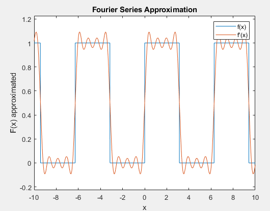
Figure 1 – B.2 Plot
3. Run the code that results from B.2 for N_TERMS = 10,20 and 30 without closing the Figure each time you run. This way you will have multiple plots on Figure 1. Include the plot on your report and answer the following question: considering the ideal square wave f(x) as a reference, where in the signal wave do the approximations of f(x) have the greatest error/oscillation?
– The greatest error occurs at the beginning of the peak of the approximate “square wave” and at the end of the peak. The peak goes too high, and then rebounds too low, then oscillates controllably until the end of the peak where it bounces high again before dropping to the inverse peak.

Figure 2 – B.3 Plot
4. The Gibbs phenomenon is an overshoot (or “ringing”) of the Fourier series. Defining the overshoot as the difference in amplitude between the highest point of the approximation and the reference function, record the overshoot values in Table 1 associated with each of the following number of terms. What is the relationship between the overshoot and the number of terms in the series?
– The relationship is the more terms there are, the less the overshoot there is.
Number of terms | Overshoot |
7 | 0.09211 |
20 | 0.08919 |
30 | 0.08345 |
50 | 0.08238 |
5. Run CODE 2 multiple times (for N_TERMS = 7, 20, 30, 50 and 100.) and, using the command tic toc, record in Table 2 the time MATLAB takes to perform the approximation of f(x). Notice that you can uncomment % tic and % toc to perform the required task. (Note: the time it takes the program to complete a set task will be different if it is the first time running the program. Take measurements after running the program once)
|
Number of terms |
Computational time |
|
7 |
0.047281 |
|
20 |
0.106378 |
|
30 |
0.147474 |
|
50 |
0.280875 |
|
100 |
60.352342 |
6. From the previous problems it could be noticed that, the higher number of terms of the series is, more precise the approximation will be; however, the computational time cost increases. In practice, we must find a balance between precision and computational cost when
using Fourier series. What determines this balance?
– The needs of whatever system that requires a signal determines the balance. Some systems may require a more precise signal with the ability to sacrifice some computational time, while others are more powerful systems that can have the same precision without sacrificing much computational time. Some systems may not need a precise signal and have less computational power, so a less precise signal can be used.
C.
1. CODE 2 implements the approximation of a square wave using Fourier series. Modify this code so that it will produce the approximation of a triangular wave (more specifically, a sawtooth wave) similar to the one shown in Figure 1. In your report, include, on the same figure, plots of the approximated sawtooth function considering N_TERMS = 10, 20 and 30.
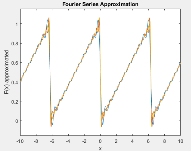
Figure 3 – Sawtooth for 10, 20, and 30
Conclusions:
This lab successfully demonstrated how a computer cannot compute a signal with infinite steps. It was found that a good number for my computer was around 30-50 terms. I enjoyed experimenting more with creating signals using the Fourier Series. I kept getting the wrong equations for the coefficients which led to the lab taking much longer than it should have. I would improve this lab by having more example signals, but providing the coefficient equations for each as to not use too much time for the lab.