Lewis Reeves
ELEC 2120 Signals & Systems
10/22/2024
Lab 8: Convolution TIMS Week 1
Introduction:
The lab demonstrates the operation of convolution using the TIMS. Students use S/H and UNIT DELAY to find the function of convolution. Students use the S&S SFP software to perform custom signals for the convolution process.
Procedure:
Part 1 –
Using the Digital Utilities, Sequence Generator, and Triple Adder modules, Figure 1 is wired into the TIMS. The clock is connected to the 1kHz lead first. Using the SFP software, the 5V signal is reduced to 1V by multiplying it by 0.247.
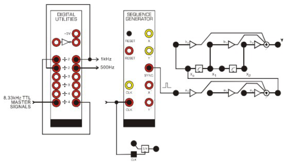
Figure 1 – System Wiring Diagram
Using the PicoScope, the output is observed showing that a periodic 1V pulse signal is output every 32 pulses as displayed in Figure 2. The signal is displayed every 32 pulses of the clock because that is how long the TIMS system delays the signal.
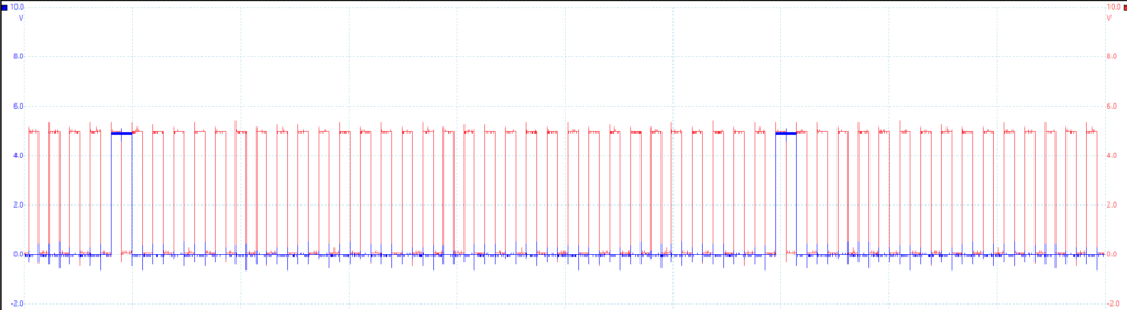
Figure 2 – One Volt Output Signal
Part 2 –
Now, in the SFP software, the gains are set to b0 = 0.3, b1 = 0.5, and b2 = -0.2. The scope inputs are switched to measuring the delay line input signal and the Adder output signal. The resulting signal is displayed Figure 3. The amplitude of each pulse in the output sequence is measured. h[0] was measured to be 0.264V, h[1] was measured to be 0.444V, and h[2] was measured to be -2.14V.
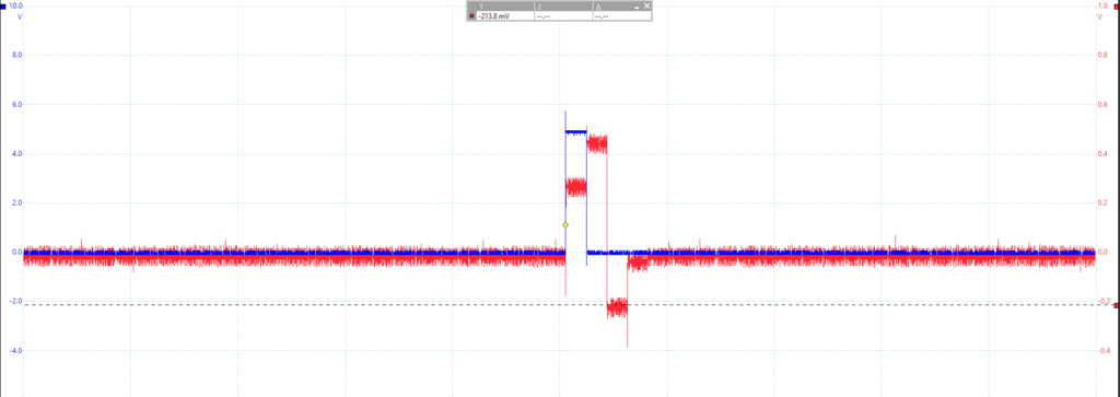
Figure 3 – Delay Line Input and Adder Output Signal
Part 3 –
The 500Hz output signal is input into the Sequence Generator clock. The 1kHz clock signal is inverted so that the 500Hz clock transitions on the positive edge of the 1kHz clock to avoid machine error. The same gain settings from Part 2 are used. The result is displayed in Figure 4.
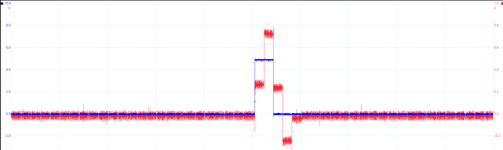
Figure 4 – Output of h[n] + h[n+1]
The graph of h[n] is displayed in Figure 5, the graph of h[n+1] is displayed in Figure 6, and the graph of h[n] superimposed on h[n+1] is displayed in Figure 7.
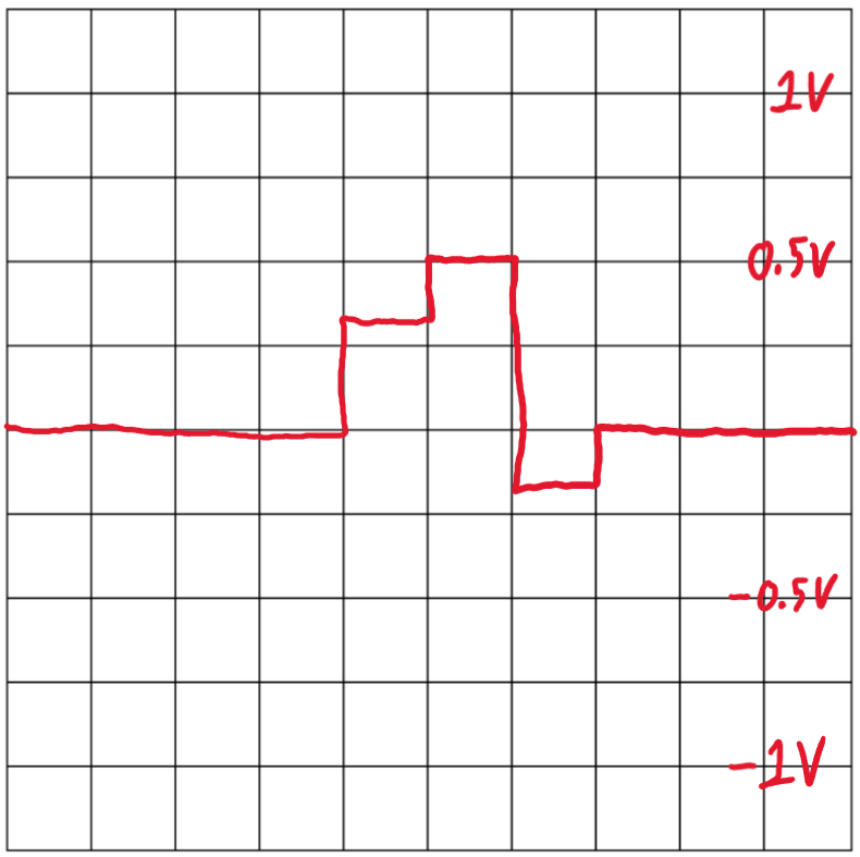
Figure 5 – Graph of h[n]
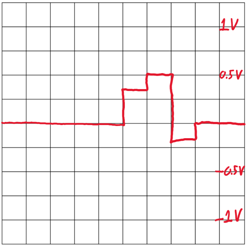
Figure 6 – Graph of h[n+1]
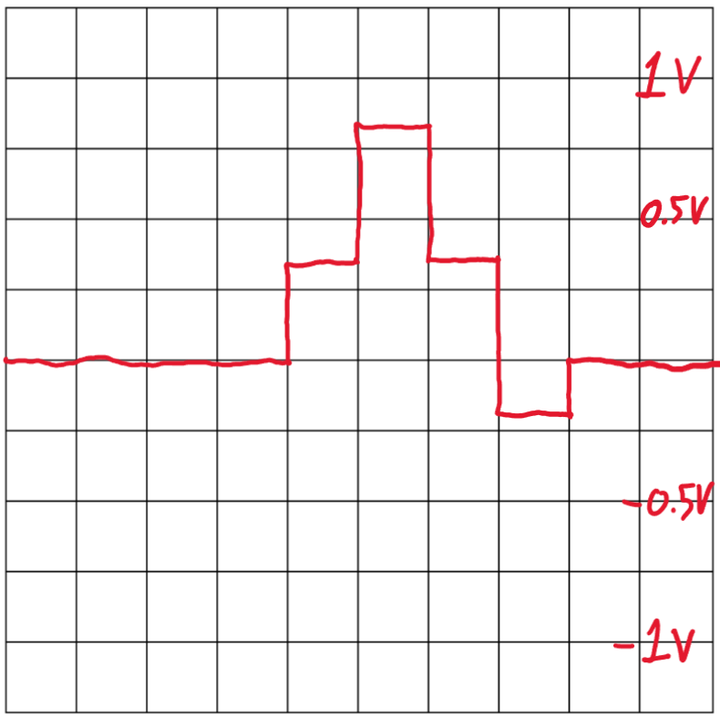
Figure 7 – Graph of h[n] Superimposed on h[n+1]
In Figure 7, the first step is seen to be the addition of the first step in both h[n] and h[n+1] which is 0 + 0.3 = 0.3. The second step is observed to also be the addition of the second step in both h[n] and h[n+1] which is 0.3 + 0.5 = 0.8. The third step is observed to be the addition of the third step of both h[n] and h[n+1] again which is 0.5 – 0.2 = 0.3. The fourth step is shown to be the addition of the fourth step in both h[n] and h[n+1] too which is 0 + 0.2 = 0.2. This successfully shows that Figure 7 is equal to h[n] and h[n+1] being superimposed onto each other.
Part 4 –
For this part, ARB1 has an output of a 100Hz sinewave at 2V amplitude which is rectified before being input to S/H, and ARB2 is a digital clock at 800Hz. The Vpp of ARB1 is measured to be 3.87V and the frequency is 100Hz. The amplitude is different because the signal is rectified before going to the S/H.
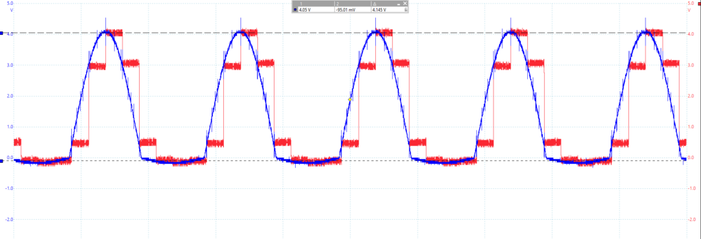
Figure 8 – Sinewave Input with S/H Discrete Output
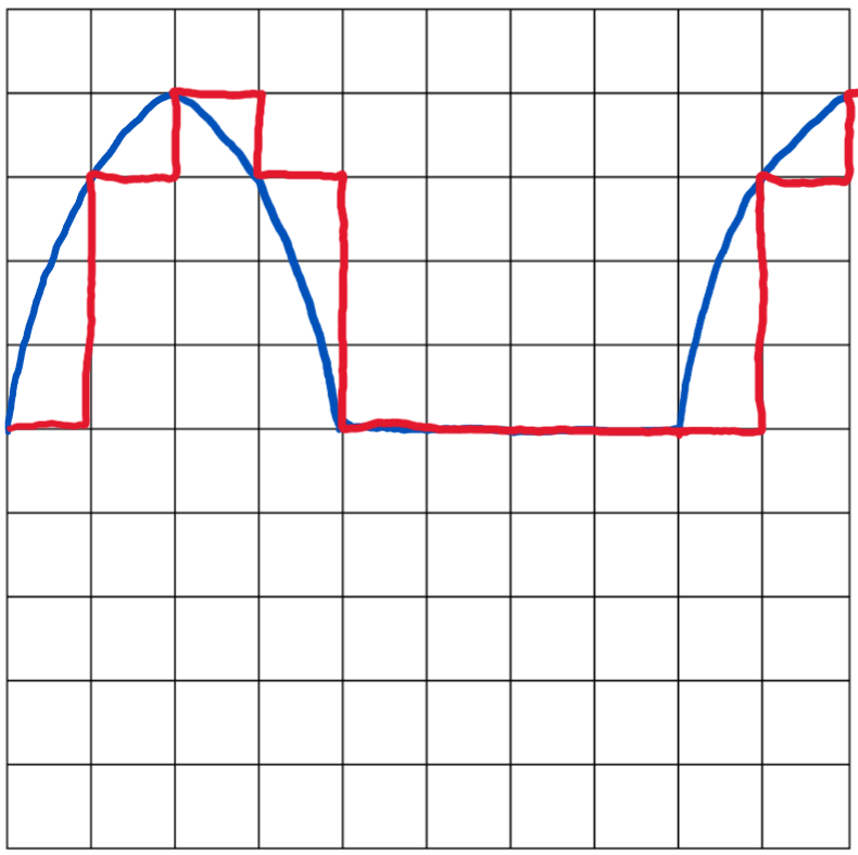
Figure 9 – Sinewave Input with S/H Discrete Output Drawing
According to the graph, the S/H function takes the input at the beginning of the period and outputs that value during the remainder of that period before outputting the next input value at the next period.
Conclusions:
This lab successfully demonstrated the function of convolution. Part 3 displayed how two functions add together to make a new signal. Part 4 demonstrated how the S/H function works in Figures 8 and 9.
I enjoyed seeing how two signals can be added together in a system. This lab was a little difficult to do because I did not understand why the inversion was necessary until thinking through the process afterwards. I would improve this lab by having more images and wiring diagrams because following this lab was more difficult than previous labs.